mlBioNets
Víctor Lázaro-Vidal
Universidad Autónoma de QuerétaroValeria Hernández Zendejas
Universidad Autónoma de QuerétaroKarel Vázquez-Suárez
Universidad Autónoma de QuerétaroRoberto Álvarez-Martínez
Universidad Autónoma de Querétaroroberto.alvarez@uaq.edu.mx
mlBioNets.RmdAbstract
Description of your vignette
Network inference
Load and preprocessing of data
# Load packages and data
library(mlBioNets)
library(phyloseq)
BN_bacter<-data(beetle_nightshade)
# Let's extract the taxonomic and abundance tables
T_table<-as.data.frame(tax_table(beetle_nightshade)); dim(T_table)
## [1] 436 7
O_table<-as.data.frame(t(otu_table(beetle_nightshade))); dim(O_table)## [1] 436 21
# The ASVs abundances are collapsed at genus level
BN_bacter2<-T_collapse(is_phyloseq = F, T_table = T_table,
                       O_table = O_table,
                       names_level = "Genus"); dim(BN_bacter2)
## [1] 21 93
# Eliminate unclassified data
BN_bacter2<-BN_bacter2[,-c(which(colnames(BN_bacter2)=="unclassified"))]

# Separate beetle and nightshade samples' ID
Insect<-which(phyloseq::sample_data(beetle_nightshade)$Type =="Insect")
Insect<-phyloseq::sample_data(beetle_nightshade)$ID[Insect]; Insect
## [1] "Eggs1" "Eggs2" "Eggs4" "Frass1" "Frass2"
## [6] "Frass3" "Frass4" "Intestines1" "Intestines2" "Intestines3"
## [11] "Intestines4"
Plant<-which(sample_data(beetle_nightshade)$Type =="Plant")
Plant<-sample_data(beetle_nightshade)$ID[Plant]; Plant
## [1] "Endophytes1" "Endophytes2" "Endophytes4" "Epiphytes1" "Epiphytes2"
## [6] "Epiphytes3" "Epiphytes4" "Seeds1" "Seeds2" "Seeds4"
# Separate abundances
Insectmat <- BN_bacter2[Insect,]
Plantmat <- BN_bacter2[Plant,]
Network inference using the SparCC algorithm
library(igraph)
# Beetle layer
library(SpiecEasi)
sparccNet<-sparcc(Insectmat)
sparccNet <- abs(sparccNet$Cor) >= 0.4
insect_sparCC<-adj2igraph(sparccNet)
vertex.attributes(insect_sparCC) <- list(name = colnames(Insectmat))
plot_network(insect_sparCC)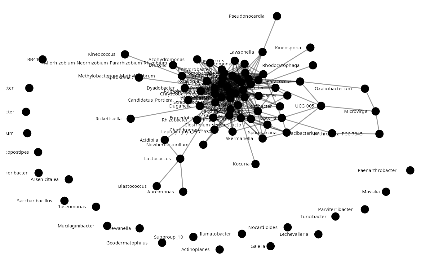
# Nightshade layer
sparccNet<-sparcc(Plantmat)
sparccNet <- abs(sparccNet$Cor) >= 0.4
plant_sparCC<-adj2igraph(sparccNet)
vertex.attributes(plant_sparCC) <- list(name = colnames(Plantmat))
plot_network(plant_sparCC)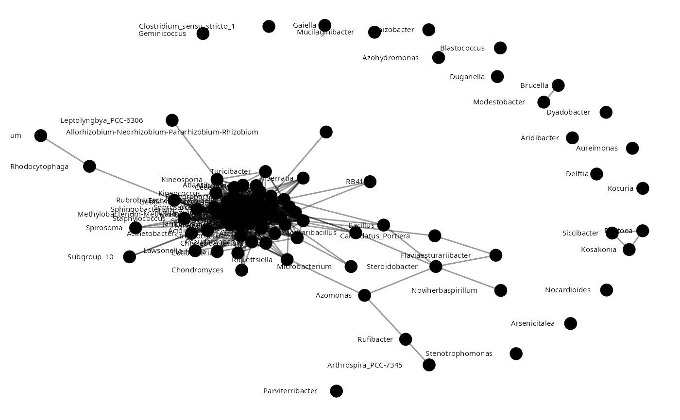
Multilayer plotting
library(muxViz)
library(viridis)

# Multilayer object
g.list<-list(insect_sparCC, plant_sparCC)
# Nodes' colors
g.list<-v_colored_ml(g.list, T_table, "Phylum", "Genus",
                     sample(viridis(100), length(unique(T_table[, "Phylum"]))))
matctr<-node_color_mat(g.list, "phylo")
# Nodes' size
matsize<-abs_mat(list(Insectmat, Plantmat), g.list, 10)
# Multilayer plot
lay <- layoutMultiplex(g.list, layout="kk", ggplot.format=F, box=T)
plot_multiplex3D(g.list, layer.layout=lay,
                 layer.colors=c("red3", "green3"),
                 layer.shift.x=0.5, layer.space=2,
                 layer.labels=NULL,
                 layer.labels.cex=1.5, node.size.values="auto",
                 node.size.scale=matsize,
                 node.colors=matctr,
                 edge.colors="black",
                 node.colors.aggr=NULL,
                 show.aggregate=F)
rglwidget()
Image 3
Network inference using ARACNe algorithm
library(minet)
# Beetle layer
mim <- build.mim(Insectmat,estimator="spearman")
Imat <- aracne(mim)
insect_aracne<-graph.adjacency(Imat)
insect_aracne<-as.undirected(insect_aracne)
plot_network(insect_aracne)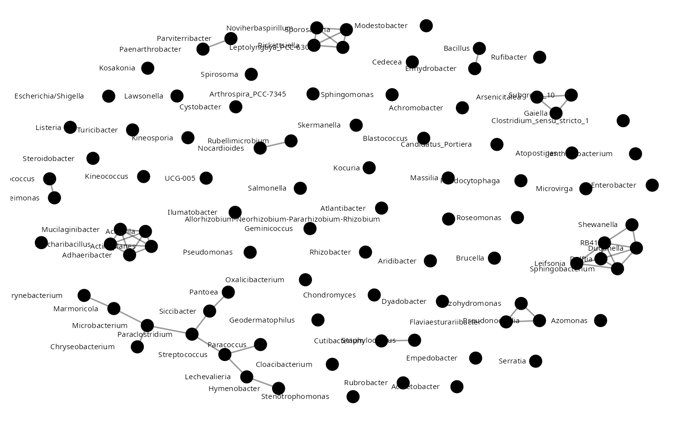
# Nightshade layer
mim <- build.mim(Plantmat,estimator="spearman")
Pmat <- aracne(mim)
plant_aracne<-graph.adjacency(Pmat)
plant_aracne<-as.undirected(plant_aracne)
plot_network(plant_aracne)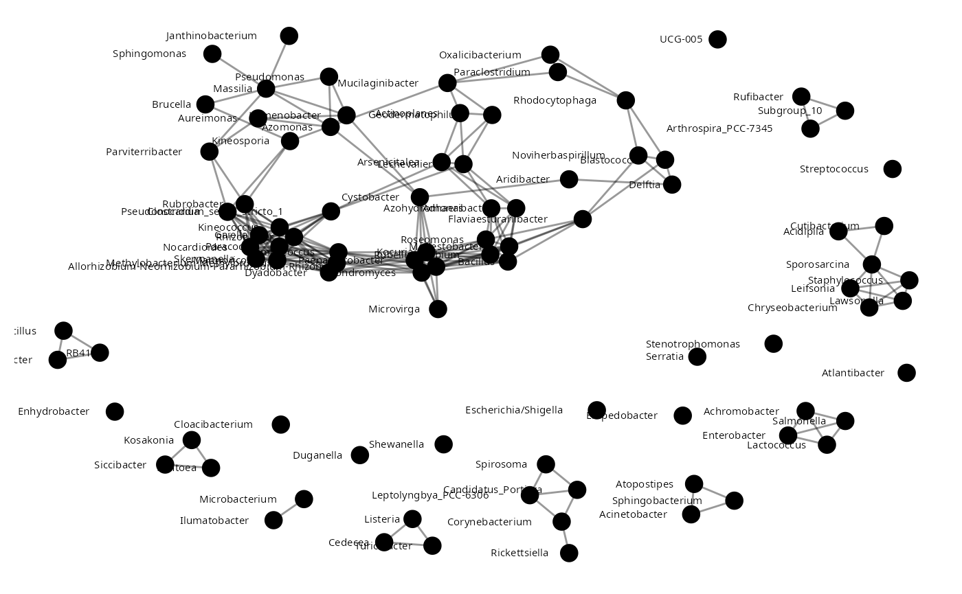
Multilayer plotting
library(muxViz)
library(viridis)
# Multilayer object
g.list<-list(insect_aracne, plant_aracne)
# Nodes' colors
g.list<-v_colored_ml(g.list, T_table, "Phylum", "Genus",
                     sample(viridis(100), length(unique(T_table[, "Phylum"]))))
matctr<-node_color_mat(g.list, "phylo")
# Nodes' size
matsize<-abs_mat(list(Insectmat, Plantmat), g.list, 10)
# Multilayer plot
lay <- layoutMultiplex(g.list, layout="kk", ggplot.format=F, box=T)
clear3d(type = "all")
plot3d_1 <- plot_multiplex3D(g.list, layer.layout=lay,
                 layer.colors=c("red3", "green3"),
                 layer.shift.x=0.5, layer.space=2,
                 layer.labels=NULL,
                 layer.labels.cex=1.5, node.size.values="auto",
                 node.size.scale=matsize,
                 node.colors=matctr,
                 edge.colors="black",
                 node.colors.aggr=NULL,
                 show.aggregate=F)
## $FOV
## [1] 30
##
## $userMatrix
## [,1] [,2] [,3] [,4]
## [1,] 1 0.0000000 0.0000000 0
## [2,] 0 0.3420201 0.9396926 0
## [3,] 0 -0.9396926 0.3420201 0
## [4,] 0 0.0000000 0.0000000 1
##
## $.position
## [1] 0 -70
Cross-references
Apart from referencing figures (Section @ref(figures)), tables (Section @ref(tables)), and equations (Section @ref(equations)), you can also use the same syntax to refer to sections by their default labels generated by pandoc.
Side notes
Footnotes are displayed as side notes on the right margin1, which has the advantage that they appear close to the place where they are defined.
Session info
## R version 4.4.2 (2024-10-31)
## Platform: x86_64-pc-linux-gnu
## Running under: Ubuntu 24.04.2 LTS
##
## Matrix products: default
## BLAS:   /usr/lib/x86_64-linux-gnu/blas/libblas.so.3.12.0
## LAPACK: /usr/lib/x86_64-linux-gnu/lapack/liblapack.so.3.12.0
##
## locale:
##  [1] LC_CTYPE=en_US.UTF-8       LC_NUMERIC=C
##  [3] LC_TIME=es_MX.UTF-8        LC_COLLATE=en_US.UTF-8
##  [5] LC_MONETARY=es_MX.UTF-8    LC_MESSAGES=en_US.UTF-8
##  [7] LC_PAPER=es_MX.UTF-8       LC_NAME=C
##  [9] LC_ADDRESS=C               LC_TELEPHONE=C
## [11] LC_MEASUREMENT=es_MX.UTF-8 LC_IDENTIFICATION=C
##
## time zone: America/Mexico_City
## tzcode source: system (glibc)
##
## attached base packages:
## [1] stats     graphics  grDevices utils     datasets  methods   base
##
## other attached packages:
##  [1] minet_3.62.0      viridis_0.6.5     viridisLite_0.4.2 muxViz_3.1
##  [5] SpiecEasi_1.1.3   igraph_2.1.4      phyloseq_1.41.1   mlBioNets_0.1.0
##  [9] rgl_1.3.17        BiocStyle_2.32.1
##
## loaded via a namespace (and not attached):
##  [1] ade4_1.7-22             tidyselect_1.2.1        farver_2.1.2
##  [4] dplyr_1.1.4             Biostrings_2.72.1       fastmap_1.2.0
##  [7] digest_0.6.37           lifecycle_1.0.4         cluster_2.1.6
## [10] survival_3.7-0          magrittr_2.0.3          compiler_4.4.2
## [13] rlang_1.1.5             sass_0.4.9              tools_4.4.2
## [16] yaml_2.3.10             data.table_1.16.4       knitr_1.49
## [19] labeling_0.4.3          htmlwidgets_1.6.4       plyr_1.8.9
## [22] withr_3.0.2             BiocGenerics_0.50.0     desc_1.4.3
## [25] grid_4.4.2              stats4_4.4.2            multtest_2.60.0
## [28] biomformat_1.32.0       colorspace_2.1-1        Rhdf5lib_1.26.0
## [31] ggplot2_3.5.1           scales_1.3.0            iterators_1.0.14
## [34] MASS_7.3-61             cli_3.6.4               rmarkdown_2.29
## [37] vegan_2.6-10            crayon_1.5.3            ragg_1.3.3
## [40] generics_0.1.3          rstudioapi_0.17.1       pulsar_0.3.11
## [43] httr_1.4.7              reshape2_1.4.4          ape_5.8-1
## [46] cachem_1.1.0            rhdf5_2.48.0            stringr_1.5.1
## [49] zlibbioc_1.50.0         splines_4.4.2           parallel_4.4.2
## [52] BiocManager_1.30.25     XVector_0.44.0          base64enc_0.1-3
## [55] vctrs_0.6.5             glmnet_4.1-8            Matrix_1.7-1
## [58] jsonlite_1.9.0          VGAM_1.1-12             bookdown_0.42
## [61] IRanges_2.38.1          S4Vectors_0.42.1        systemfonts_1.1.0
## [64] foreach_1.5.2           jquerylib_0.1.4         glue_1.8.0
## [67] pkgdown_2.1.1           codetools_0.2-20        shape_1.4.6.1
## [70] stringi_1.8.4           gtable_0.3.6            GenomeInfoDb_1.40.1
## [73] UCSC.utils_1.0.0        munsell_0.5.1           tibble_3.2.1
## [76] pillar_1.10.1           htmltools_0.5.8.1       rhdf5filters_1.16.0
## [79] huge_1.3.5              GenomeInfoDbData_1.2.12 R6_2.6.1
## [82] textshaping_0.4.1       evaluate_1.0.3          lattice_0.22-6
## [85] Biobase_2.64.0          bslib_0.9.0             Rcpp_1.0.14
## [88] gridExtra_2.3           nlme_3.1-166            permute_0.9-7
## [91] mgcv_1.9-1              xfun_0.51               fs_1.6.5
## [94] pkgconfig_2.0.3